
walking-client
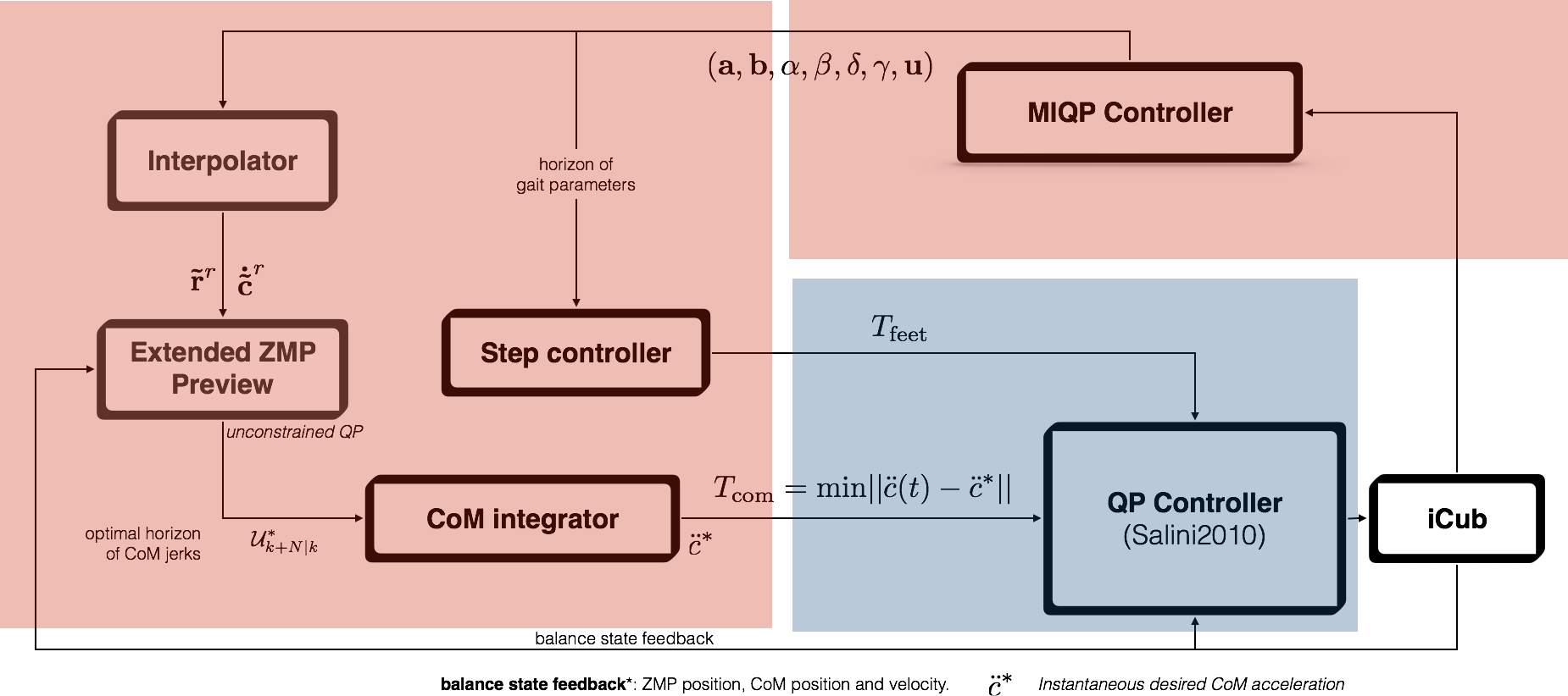
The walking-client is an implementation of a predictive approach [1] to preview the duration and placement of coplanar feet contacts of the iCub humanoid robot exploiting the OCRA framework. Within a model-predictive control (MPC) framework, the problem is formulated as a linearly constrained mixed-integer quadratic program (MIQP) which allows the determination over a preview horizon, of the optimal changes in the base of support (BoS) of the robot with compatible Center of Mass (CoM) behaviour, subject to multiple constraints, while maximising balance and performance of a walking activity.
The following sections can be seen as an addendum to [1] which gives a detailed insight of the MIQP formulation. It assumes that the reader has gone through [1] (or at least Chapter 5) and needs more details for understanding the nuances of the client
walking-client. For more theoretical and complementary information, refer to the thesis itself.
The walking problem can be be seen as a compromise between CoM trajectory tracking and balance. By using the CoP distance from the boundaries of the BoS as the indicator for balance performance and CoM tracking error as the one for walking performance, plus the addition of suitable constraints with integer and real variables, the walking problem writes:
The MIQP canonical form of the cost function originates from the following cost function:
which represents the formerly described compromise between the walking ($J_{w_k}$) and balance ($J_{b_k}$) performances, i.e.
Where $q$ are regularization terms. More details later on.
Let’s work out a bit more Equation \ref{eq:miqpEquation} before moving to the details of the regularization terms and constraints.
The global cost function (without regularization terms) can be written in matrix form as:
Where, in the walking performance cost, is the vector of predicted CoM outputs in a preview window of size $N$, while is the vector of CoM state references in the same window. On the other hand, is the vector of predicted CoP outputs and , the vector of predicted BoS centers.
Given the system state (more on this in [1] Sections 5.1.2, 5.2) and input $\mathcal{X} = (\mathbf{a} \; \mathbf{b} \; \mathbf{\alpha} \; \mathbf{\beta} \; \delta \; \gamma \; \mathbf{u} )$, we can predict the CoM outputs in a preview window ($\mathbf{H}_{k,N}$) from the state propagation:
Where
and the relationship between the system and CoM state, i.e.
Where:
Then by iteratively applying the previous system of equations, we arrive to the following compact matrix expression:
Where:
We will call matrices like $\mathbf{P}_H$ and $\mathbf{R}_H$, preview state and preview input matrices respectively.
We need to proceed in a similar fashion as before to obtain an expression for the predicted CoP outputs in the preview window. So, again, keeping in mind that:
And that in this case:
Where, assuming a simplified Linear Inverted Pendulum model of the robot and constant CoM height $c_z$:
We can thus obtain a compact expression for $\mathbf{P}_{k,N}$ as:
Where $\mathbf{P}_P$ and $\mathbf{R}_P$ have the same structure as $\mathbf{P}_H$ and $\mathbf{R}_H$ but using $\mathbf{C}_P$ instead of $\mathbf{C}_H$.
Once more we look for an expression for the predicted BoS outputs in the preview window, but this time:
Where:
We can again obtain a compact expression for the predicted BoS outputs:
By replacing the previous CoM (\ref{eq:comPrediction}), CoP (\ref{eq:copPrediction}) and BoS (\ref{eq:bosPrediction}) predicted outputs in the matrix form of the cost function (\ref{eq:costFuncMatrix}) we get:
For the first part of the cost function given the symmetry of some resulting terms and getting rid of some subscripts to simplify the writing:
The first term in (\ref{eq:firstTermCompact}) is not a function of $\mathcal{X}$ and therefore won’t make part of the final cost function.
Expanding the second part of the original cost function, i.e. and again exploiting the symmetry of some resulting terms:
Adding up (\ref{eq:firstTermCompact}) and (\ref{eq:secontTermCompact}) (only those terms which are function of $\mathcal{X}$) we get:
Which gives the final expression for the cost function:
Where:
A few regularization terms (or secondary objectives) in the cost function (\ref{eq:costFunction}) are necessary in order to:
These costs are quadratic and the ones already implemented are described below:
This cost prevents the resulting CoM jerks to be too large and writes:
Which can be further elaborated in terms of the input vector $\mathcal{X}$ and optimization variable $\mathcal{X}_{k,N}$ as:
Where:
while:
Finally, Eq. (\ref{eq:jerkPreview}) can be added to Eq. (\ref{eq:finalCostFunction}).
In order to avoid resting on one foot, the following cost function is added:
For a preview window of size $N$ in matrix form this writes:
Then, as done in the previous sections for the prediction of CoM, CoP and BoS given that:
Where:
An expression for $\mathbf{\Gamma_{k,N}}$ can be found:
Where and are similar to (\ref{eq:previewStateMatrix}) and (\ref{eq:previewInputMatrix}) using instead .
By substituting Eq. (\ref{eq:gammaPreview}) in Eq. (\ref{eq:supportPhaseRegCostMatrix}) we get:
Which in this form can then be added to Eq. (\ref{eq:finalCostFunction}).
These regularization terms aim at the minimization of stepping and writes as:
For a preview window of size $N$ in matrix form this writes:
Then, given that:
Where:
Thus, for the preview window we have:
Which allows us to write this cost function in terms of the input $\mathcal{X}$
Not implemented yet
Not implemented yet
The constraints of the MIQP problem (\ref{eq:miqpEquation}) at this moment contain three types of constraints:
All constraints are linear. The following sections do not provide an explanation of what each constraint is, but shows only the corresponding matrix expressions later used in walking-client. For further information, refer to [1]-Appendix B.
These consist at time step $i$ of:
Bounding:
Constancy:
Sequentiality:
These constraints have a similar structure, depending either on the the current state only or also on the next system state. Therefore Shape Constraints at time step $i$ can be expressed in a compact form as:
In Eq. (\ref{eq:bounding})
and
In Eq. (\ref{eq:constancy})
And
In Eq. (\ref{eq:sequentiality})
These consist at time step $i$ of:
Single and Double Support Alternation
Single Support
Contact Configuration History
Contact Configuration Enforcement
These constraints have a similar structure, depending either on the the current state only or also on the next system state. Therefore Admissibility Constraints at time step $i$ can be expressed in a compact form as:
In Eq. (\ref{eq:SDSAlternation})
And
In Eq. (\ref{eq:singleSupport})
and
In Eq. (\ref{eq:contactConfigHistory})
and
In Eq. (\ref{eq:contactConfigEnforcement})
Recalling the preview model (\ref{eq:previewModel}) we can obtain an expression for the constraints matrices in the preview window as done for the CoM, CoP and BoS in previous sections. Thus, stacking inequalities (\ref{eq:shapeCompact}) and (\ref{eq:admissibilityCompact}) by denoting:
We have shape and admissibility constraints at time $i$ in compact form as:
We need however to write these constraints in the preview window and in terms of the optimization variable $\mathcal{X}$ as
Thus, by iteratively applying Eq. (\ref{eq:shapeAdmissCompact}) for $i\in[k,N-1]$ we get:
While:
In this approach the convex hull is overestimated by its bounding box and defined by the minimum and maximum points as shown in the next image:

These constraints write in terms of the CoP $\mathbf{p}$:
or $\mathbf{A}_b\mathbf{p}\leq\mathbf{b}$, and in terms of the system state as:
Where:
and
Then, in a preview window, given preview model (\ref{eq:previewModel}) and iteratively applying Eq. (\ref{eq:bboxConstraints}) we get the following set of constraints:
Where:
While:
The simplest test that can be done with the MIQP controller is to provide a CoM velocity reference that would move the robot either left or right on one foot, having at least:
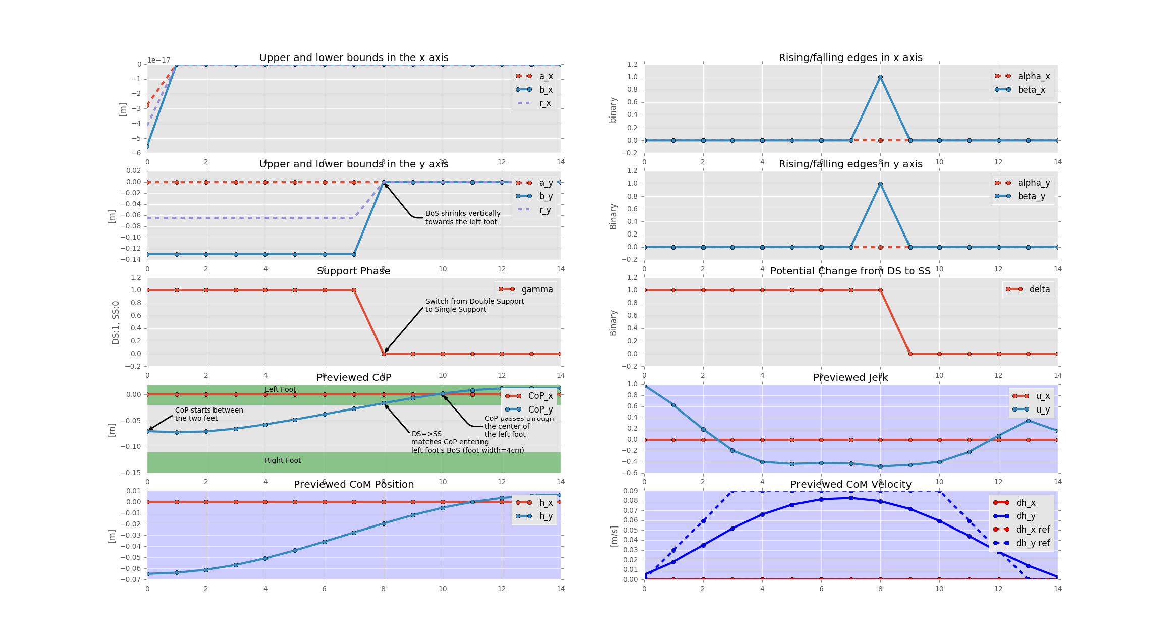
Most of the important annotations/observations have been put in the image above, where the following parameters in walking-client.ini have been used:
[MIQP_CONTROLLER_PARAMS]
robot icubGazeboSim
dCoMxRef 0.0
dCoMyRef 0.09
N 15
wb 1
ww 3
wu 0.3
wss 0.001
wstep 0.01
wdelta 0.0001
g 9.8
dt 100
dtThread 100
sx_constancy 0.3
sy_constancy 0.3
sx_ss 0.3
sy_ss 0.3
hx_ref 0.0
hy_ref 0.0
dhx_ref 1.0
dhy_ref 1.0
ddhx_ref 0.0
ddhy_ref 0.0
marginCoPBounds 0.008
shapeConstraints true
admissibilityConstraints true
copConstraints true
walkingConstraints false
addRegularization true
[1] Ibanez A. Ph.D. thesis